Thevenin's Theorem Lab

Objective:
The goal of today's class meeting is to understand Thevenin's Theorem. Thevenin started working in the telegraph service and eventually became the chief inspectors of the telegraph service. When applying Thevenin's Theorem, a linear two terminal circuit can be replaced by an equivalent circuit that includes the Rth and Vth.  When finding the Rth, we turn off all independent sources and find the Req. Finally we can acquire the Vth at the terminals where their is an open circuit.

Group Practice:
1. The image below shows a practice problem in which we are finding the Rth using Thevenin's Theorem. We can see that the Rth= 10 ohms. We acquire this value by replacing the voltage and current sources with a line, thus turning them off and find the Req which is the Rth.

Figure 1. In class work in which we find the Rth

2. The second in class problem involves another circuit in which we found the Rth = 12 ohms and Vth = 40v by using Thevenin's Theorem.

Figure 2. In class work in which we find the Rth and Vth in a circuit by applying Thevenin's Theorem.

Lab Procedures and Results:
1. The lab involves the use of Thevenin's Theorem where we compare our theoretical values of Rth and Vth with our experimental values of Rth and Vth. In order to start with our experiment, we will calculate the theoretical Values of RL and VL as seen in Figure 3. We note that the 1.5K resistor will be replaced by a 1.8K resistor since it is the only resistor available in class.

Figure 3. Schematic of circuit where the 1.5K resistor is replaced with a 1.8K resistor.

2. The values of Rth = 7.7K and Vth = .4579V as seen in Figure 4.

Figure 4. The visual solution for Rth and Vth. 

3. The next step is to create the circuit from figure 3. The actual circuit can be seen below. The actual resistance measure by the digital ohmmeter are R1K = .96K+/-.01, R4.7K = 4.6K+/-.05, R6.8K=6.66K+/-.01, R1.8K = 1.75K+/-.01, R6.8K = 6.8K+/-.01, and R2.2K=2.16K+/-.01.

Figure 5. The actual Circuit setup for experimenting on Thevenin's Theorem

4. We measure the voltage across the terminals a-b and make sure that there is an open circuit for RL. the The voltage is Vth = .46V+/-.01 and can bee seen in Figure 6 below. The Rth is measured to be Rth = 7.4K+/-.01 which can be seen in Figure 7. The way we measure the Rth is by setting the voltage sources to short circuits.

Figure 6.

Figure 7. 

5. We then pick a random resistor of R4.7K = 4.54K+/-.01 within the range 4k<RL<10K and connected to the terminals a-b. We measure the voltage across the resistor and get a VRL=7.4K+/-.01 which can be seen in Figure 8. below. We notice that we acquire the same thevenian voltage which is what we expect based on the theorem.

Figure 8. The measure voltage of Vth using a 4.7K resistor.

Figure 9. Percent error between theoretical and experimental values.

6. The last step is to connect the potentiometer between the terminal a-b. We measure and record the load function and the potentiometer resistance as seen in figure 10. We will also create a powers vs load resistance plot using only 4 measurements. We expect to reach a max power output and then drop at some point.

Figure 10. Measurements of voltage and resistance, as well as the calculations for power. 

Figure 11. Power vs load resistance plot. 

Summary of Lab and Learning Outcome:
The purpose of the lab is compare our theoretical and experimental values of Rth and Vth. Out comparison shows that Thevenin's theorem is precise based on the values that we calculated and measured which can be seen in figure 9. We see that we acquire a percent error of 3.89% for the Rth and .459% for the Vth. The low percent error satisfies our expectations of Thevenin's theorem. A potentiometer is also connected where the Rth is located which can be seen in figure 3. We then measure the voltage across the terminal a-b. The measurements are plotted in a power vs load resistance plot which can be seen in figure 11. We see that the power increases and reaches a maximum power of 6.22 micro watts, a voltage of .22V when the resistance is 8.5K.

Superposition 2 Lab

Objective:
We are introduced to Every circuit which helps analyze and simulate a circuit. This chrome application is helpful to understand the values at each resistor or other unknown currents and voltages. We are also introduced to a new method called linearity which its output is linearly related or directly proportional to its input. In other words, the linearity property says that when the cause changes to some amount, the effect changes to the same amount. Finally we deal with superposition and transformation which are methods that make circuit analysis easier to calculate in terms of what we are finding.

Group Practice:
1. The image below shows voltage and current independent source on each side of the circuit and are told to find the current flow through the 5 ohm resistor. In order to accomplish this, we use superposition which is method that enables the current source to be set to zero or voltage to zero. However, it must be done once at a time at each side. Then we acquire the currents and them together as seen in Figure 1.

Figure 1. Superposition class work

Superposition Lab Procedures and Results:

1. In this lab, we must first find theoretical value of voltage by using superposition as seen in figure 2. First we set the voltage source of 3V to zero and find the voltage V1 = 2.2V using current division. Then we set the voltage to the right to zero and find the voltage V2=.71V from that source. Finally we add the voltages V = V1+ V2 from both independent sources. We get a theoretical value of V = 2.9V which seem to be too high but will compare to our experimental value of voltage at 6.8k resistors.

Figure 2. Finding the theoretical voltage at the 6.8k resistor

2. We commence to build our circuit based on the schematic in Figure 3. We notice that we don not have a 20 kilo ohm resistor available in class and change it to a 22k resistor since it is what we have in class and because this value was used to find our theoretical Voltage at the 6.8 resistor.

Figure 3. Schematic for a circuit with two independent voltage sources. 

3. We record the actual resistance of the resistors: R10K = R4.7K = R6.8K = R22K = R1K =

4 . We measure the voltage across the 6.8k resistor while the 3V source is replaced with a short circuit and measure a value of V1 = .69V +/-.01

Figure 4. Value of voltage for V1

5. We measure the voltage across the 6.8k resistor while the 5V sources is replaced with a short circuit and measure a value of V2 = 1.98V +/-.01

Figure 5. Value of voltage of V2

6. We then measure the voltage at the 6.8k resistor with both voltage sources in place and find a value of V = 2.69V +/-.01

Figure 6. Total voltage at the 6.8k resistor

Figure 7. Values for V1 and V2

Summary of Superposition Lab and Learning Outcome:

The theoretical values for voltages V1 and V2 while each of the independent voltages sources are equal to zero correlate and match with our experimental values. We see that their is a low percentage of error for V1 % error = |(2.2-1.98)|/2.2 *100= 10% and V % error = |.71-.69|/.71*100 = 2.8%. Their true Voltage error at the 6.8k resistor is % error = |(2.9-2.69)|/2.9*100 = 7.24%. We can agree that superposition is theoretically correct and serves beneficial for reducing complex circuits to simpler circuits. The final tables with results and percentage error may be seen in figure 7 above. 

Mesh Analysis 2

Objective:
The goal is to understand the difference between nodal and mesh analysis. Nodal analysis is easier with current sources and mesh analysis is easier for voltage sources. If we are asked to find the currents in a circuit, then we would use mesh analysis. If asked to find voltages, we use nodal analysis. The main key is to use the easiest method for which will acquire the least number of equations. We are also introduced to transistors which are modeled as active devices. Furthermore, we will learn how to do circuit analysis of transistors and time based analysis (Time based measurements).

Group Practice:
1. The first problem that we worked on required the use of mesh analysis as seen in Figure 1. We used 3 mesh currents i1, i2, and i3 and used ohms law to express the voltages. However, We learned a new and easier way to solve the problem as seen in Figure 2.

Figure 1. A circuit problem in which mesh analysis is used. 

Figure 2. A new way of solving for the currents without much calculations. 

2. In figure 3, we have a transistor circuit and are told to find the Ib, Ic and Vo. In order to start, we need to create an equivalent model as seen in figure 3 below the first model. We use mesh analysis and find that Ib = .165 mA, we find Ic = BIb = 50(.165) = 8.25mA. Finally we find V0 by using mesh analysis where -V0 -100(.00825)+6 = 0, so V0 =5.18V 

Figure 3. Calculations for Ib, Ic , and Vo in a transistor circuit.

Mesh Analysis Lab Procedures and Results:
1. In order to start with our experiment, we calculated the theoretical values for V1 and I1 as seen in Figure #. We acquired values of V1 = 5.018V and I1 =-.322mA using mesh analysis and solving for the currents using MATLAB as seen in Figure 5. Though, it is important to note that our resistance for the 20 kilo ohm resistor was changed to a 22 kilo ohm resistor since it is the only closest resistance for a resistor in class.

Figure 4. Theoretical calculations for V1 and I1

Figure 5. Matlab is used to find the currents of the three meshes seen in Figure 4.  

2. We constructed a a circuit as seen in figure 6. However we first measured actual resistance values from our resistors used which are: R20K = 21.6K=/-.05, R10K =9.7K+/-.05, R4.7K = 4.5K+/-.05, R6.8K = 6.5K+/-.05.

Figure 6. Schematic of circuit in which the resistance of the resistors are not within the actual values.

3. The experimental measurements are V1 = 4.96+/-.05 and I1 =-.318 +/- .05 in the circuit.

Figure 7. Resistance of I1

Figure 8. Voltage of V1

4. Based on our theoretical and experimental measurements, we can calculate for the percent error where % error = | (experimental-theoretical) | / theoretical * 100 . Our percent error for Voltage is 1.15% We can see that out theoretical calculations does accurately fall within our experimental measurements since our percent error is low. 

Time Varying Signals Lab Procedures and Results:
1. We practiced using a arbitrary waveform generator to generate time varying signals.
2. We set a circuit where there is a voltage divider as seen in Figure 9 and 10.

Figure 9. A circuit where there is a voltage divider relation

Figure 10. Using Oscilloscope to measure varying signals

Summary of Labs and Overall Learning Outcome:

The schematic of the circuit with meshes and values may be seen in Figure 4 with the use of Matlab calculations for currents in Figure 5. We acquired theoretical measurements of V1= 5.018 and I1 =-.322mA . From our experimental measurements, we acquired values of V1 = , I1 =, and actual resistance values for each resistor where R20K = 21.6K=/-.05, R10K =9.7K+/-.05, R4.7K = 4.5K+/-.05, R6.8K = 6.5K+/-.05. We can concluded that our theoretical values do not have a significant difference with our experimental measurements since the percent error was a low 1.15% for voltage at V1 and a low 1.36% for current at I1. Using mesh analysis does in fact show useful and accurate values in a theoretical manner. In the end of class and for the last ab of the day we used the Oscilloscope to measure a varying signal from a voltage divider as seen in Figure 9 and 10.

Nodal Analysis Lab

Objective:
The goal is to review nodal voltage analysis for which will helps us find a system of linear equations. From the system of equations, we can use the the idea of Ax=B and use Cramer's Rule or use other methods of finding the voltages such using the reduced row echelon. From this idea, we will build a circuit for our lab containing multiple sources for which we can apply nodal voltage analysis. Furthermore, we covered mesh analysis which is another way of doing circuit analysis. The idea is to
define a mesh when a loop with loops that go clockwise because of convention so that results are all the same for the classroom.

Group Practice:
1. We apply nodal voltage analysis for Figure 1 as seen below in order to acquire all the voltages at the nodes. Figure 1 does not give the correct answers since we did not have correct voltage direction. Figure 2 shows how to set the equations correctly and may find the unknown voltages at the nodes using Kramer's rule or Gaussian elimination.

Figure 1. The images shows a circuit where nodal voltage analysis is used. 

Figure 2. The image shows the correct way to set up a system of linear equations for the first practice problem worked in class. 

Lab Procedures and Results:
1. The focus of the lab is to use nodal analysis for Figure 3 to predict the circuit behavior before we build and test the circuit with what we have available in class. We will then compare our experimental results with our theoretical results to find the percent error.

2. We acquired a theoretical voltage of V1 = 2.42V and V2 = 4.4241V by using nodal voltage analysis in Figure 4. Note: We used a 20K resistor at V2 since it was the only one available and near to the value.

Figure 3. A circuit that is used to predict and then test for the voltages at V1 and V2. 

Figure 4. Our predicted results for V1 and V2

3. The next step is to physically build the circuit as seen in Figure 4 by following the circuit schematic in Figure 3. It is crucial to point out that we did not use 20K resistor since the value of that resistor was not available to us. Instead, we used 22k resistor. We can see that the circuit has parallel resistors and voltage sources for which we included in our build. We note that the red wire represents the +5V, white as -5V, and yellow as -3V from our analog discovery box. The -3V was programmed through the waveform tab while the +5V and -5V are automatically outputting voltages. 

Our exact values for resistors are 9.8K, 21.8K, and 6.72K.

Figure 5. Actual circuit testing and connection as seen from Figure 3. 

3. The experimental measurements for V1 = 2.43+/-.05V as seen in Figure 6 and V2 = 4.39V+/-.05 as seen in Figure 7. By comparing our theoretical values of  V1 = 2.42V and V2 = 4.4241V and experimental values of V1 = 2.43V and V2 = 4.39, we can see that our results were fairly the same. 

Figure 6. A measurement of 2.43V for V1.

Figure 7. A measurement of voltage of 4.39V for V2. 

4. Finally, we calculate the percent error for each voltage where % error = abs((experimental-theoretical)/theoretical)X100. The percent error for V1 is % error = | (2.43-2.42)/2.42 |*100= .41%

The percent error for V2 is % error = | (4.39-4.4241)/4.4241 |*100 = .77%

Summary of Lab and Overall Learning Outcome:

We can conclude that our theoretical values are accurate to our experimental measurements which means that the nodal analysis holds true to its name. Though, our true resistance measurements were not the same as the theoretical values of the resistors, we found that there is a percent error between them where V1 had .41% error and V2 a .77% error. Since the percent error is below 1%, we are satisfied with the idea of using nodal voltage analysis for calculating for the unknown voltages at any node. 

MATLAB Practice

Objective. 

The reason for introducing MATLAB to the class is to make our calculations easier to acquire since we are dealing with circuits who have many unknown currents or voltages in the form of a system of equations. We can place theses equations into matrices and solve for the unknown using the reduced row echelon or using the matrix inverse. We will use all the skills from the MATLAB practice packet for our future problems involving circuits. 

MATLAB Codes and Results:

The images below shows the use of percentage sign to signify that there is comment written with the particular problem or exercise. The answer is also shown on the right of some of the images. However, Some of the problem answers were too long to show so they had to be suppressed. Overall, Matlab makes problem solving easier than doing on paper and saves time. I also used %% to make a page break or else the results would all show from each exercise. It helps with organization and to understand the results based on the problems seen on the right highlighted in yellow.

Figure 1 The image simple math functions and the use of creating arrays. We can also manipulate the array by using the (') to transpose the array. 

Figure 2. The images above shows the use of addressing arrays and using RREF on matrices for finding unknown values. Furthermore, the image shows how to create plots with appropriate title and axis labeling. 

Figure 3. The image above goes along with Figure 2 problems as part of plotting exponentials and sinusoids. 

Figure 4. The image shows the use of adding sinusoids and conversion between rectangular to polar and vise versa. 

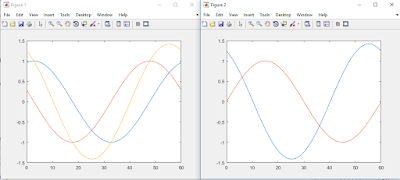
Figure 5. The image shows the plot when adding a cosine and sine function. Unfortunately, it is difficult to read which function in which. However, it can be seen more clearly in Figure 6 since a legend was introduced in the plot. 

Figure 6. The image shows the plot of circuit outputs.

Figure 7. The image shows how to convert rectangular to polar. and solving for roots of equations. 

Figure 8. This images is part of Figure 7 problems where not only the MATLAB results needed to be shown but also the theoretical results as seen above.

MATLAB Summary and Learning Outcome:

The most important outcome learned was the use of solving for the roots of equations for which would be later used for time analysis of a circuit. It is also helpful in solving a system of linear equations. Using the program has substantially increase problem solving performance. Not only is it helpful for problem solving but we are able to create our own functions or equations that may be saved for future use such as conversions. By calling the function, we can easily solve a problem depending what equation is needed to solve the problem. 

Temperature Measurement System Lab

Objective: 
Solving for unknowns needed the use of KVL or through element voltages which becomes longer work of problem solving based on the number of equations created. Instead, we are introduced with a new method called the Node Voltage Method where we find nodal voltages and ignore voltage sources. However, we are introduced with ground in a circuit which is also known as a reference node that has zero potential. We apply the equation (i = (V high-V low)/R) depending on the current we are looking for across a resistor. However we must also apply KCL to generate the needed equations. Overall, the Nodal Voltage Methods simplifies things by reducing the number of equations. We are also introduced to Super nodes which is created by having a voltage source whether dependent or independent and connected between two non reference nodes. We can then apply KVL on the super node. With this in mind if there are, for example 3 unknown, then we will need 3 equations which can be solved in MATLAB. We will use this program for the Temperature Measurement System Lab and for future use in other lab.
voltage divider
cheapest temperature

Group Practice Problems:

1. The problem in Figure 1 was a quiz question that had to be completed in 10 minutes. Unfortunately, we did not finish it on time. We figured it would take a long time. However, we were introduced to the Nodal Voltage Method which simplifies the number equations and make this problem easier to solve. 

Figure 1. The image shows a quiz question where our team had to find the voltage at R1.

2. The problem in Figure 2 shows how use the Node Voltage Method where we pick 3 node voltages and reference point where the ground connects. From this we apply the equation: i = (V high-V low)/R at each node voltage. We then apply KCL. The rest of the problem is just plugging the current to the KCL equations. Our first attempt did not go so well as seen below in figure 2 since we forgot to include one of the current when using KCL. Yet, we found the mistake and fixed it.

Figure 2. The image above shows a new method of find currents when there is ground called Node Voltage Method.

Temperature Measurement System Pre Lab and Actual Lab Procedures:

1.  Before we begin with the experiment, we start a pre lab where we are asked to find the V out and the resistance, given a input voltage of 5V as seen in figure 3. . However, the value R has to chosen carefully so that Vout increases by a minimum of .5V over the temperature range of 25C-37C. In order to find the Rth between

2. We begin our calculations by first find the resistance of the thermistor given the temperature by looking at the temperature resistance curve as seen in figure 4. We see that there is a voltage division in the circuit in figure 3. Therefore, we acquire an equation for output where V = I R where I = 5/(R+Rth). So, our equation will be Vout=R*5/(R+Rth). Since we want a voltage difference output of .5, then we create an equations where Vout(Final)-Vout(initial) = .5. Out results can be seen in Figure 5 where we acquire a quadratic equation. Finally we entered our quadratic equation  into MATLAB as seen in Figure 6. in which we acquire a theoretical resistance of 4338<R<17633. 

Figure 3. The image above shows a circuit where Rth represents the thermistor. 

Figure 4. The graph shows a temperature-resistance curve where the thermistor is used in the circuit. We see that the resistance changes as a function of temperature. 

Figure 5.  The image shows the calculated results for find the Theoretical resistance. 

Figure 6. Calculating the Resistance needed in order to acquire a voltage difference of .5V in MATLAB

3. We acquired a theoretical resistance of 4338<R<17633. However in order to create or set up our circuit we need to find a reasonable resistance provided with what we have in class. We chose a resistance of 10k since it ranges between our theoretical resistance values. The actual resistance of fixed resistor is R= 9.84+/-.05k 

4. We also measure the resistance of the thermistor at room and body temperature. The thermistor resistance at room temperature of 25C is Rth= 10.5k+/-1 and thermistor resistance at 37C is Rth= 7k+/-1 when covered with our fingers representing bod temperature of 37C.

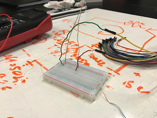
5. The circuit can be seen in figure 7 and voltage output measurement were taken when applying the thermistor at room temperature and body temperature. We acquire a measurement of Voltage output at low temp V= 2.40V and voltage output at body temperature of V = 2.93V. A video is provided that demonstrates the operation of our circuit, link: https://youtu.be/6BJOS9yp6gs

6.  We see that the difference between the voltages are Vdiff = 2.93- 2.4 = .53 which is close to what we expect to get for output voltage difference of .5 V. The percent error for voltage output difference is 6% based on the formula of percent error= |(experimental - theoretical)/ theoretical|*100.

Figure 7. Circuit setup for Temperature Measurement System.

Summary of the Lab and Overall Learning Outcome:

Our pre lab calculations tells us to find the theoretical resistance needed so that the voltage difference output is .5V. We acquire a theoretical resistance of 4338<R<17633 with the help of MATLAB. We picked a resistance of 9.84k provided by what we have available in class. We measure resistance of thermistor at room temperature 25C, R= 10.5k+/-1 and at body temperature 37C , R =7k+/-1. We can see that as temperature increases for thermistor, then resistance deceases which is what we expect based on the the graph provided in figure 4. As the thermistor increases in the temperature then we expect a high output voltage. Our results show our expectations since voltage output at body temperature was 2.93V+/-.05 compared to 2.40V+/-.05 when temperature at the thermistor was at room temperature. We acquire a 6% error which shows that our circuit performance compared well with our expected results.