Impedance Lab

Objective:
We covered phasor relationships for circuit elements. Based on the acronym "ELI the ICE man", we are able to see what value leads what. For instance, ELI means that for an inductor, the voltage leads the current. For ICE, in terms of dealing with an inductor, the current leads the voltage. Finally, for the resistor, the voltage is in phase with the current. The following are the voltage current relations for three passive elements: V=IR for resistor, V = jധLI for an inductor, V = I/jധC for a capacitor. Theses equations can then be written in terms of a ratio of the phasor voltage to current in terms of Z which represents the impedance. the impedance may be represented in rectangular form, Z= R+jX where R is the resistance and X is the impedance of the element being dealt with. We can then apply this to Kirchhoff's Laws in the Frequency Domain.

Group Practice:
1. The problem below shows a voltage source of 10cosωt connected in series with a resistor of 5Ω and a capacitor of .1F. We write the impedance and solve for it as seen below. We also solve for the current by using I=V/Z where the Z is changed to polar form. It is easier to divide using polar form. We now solve for the voltage across the capacitor using equations V = IZc. The final results will be in the time domain.

Figure 1. Solving for the current and the voltage across the capacitor.

2. The same situation is modeled as in figure 1. However, there is a current source and a capacitor to deal with. We solve for the impedance

Figure 2. Solving for voltage across the capacitor involving a current source.

3. The problem below shows a circuit with an inductor parallel to a capacitor. In order to solve this, we need to find the impedance of the elements and find their equivalent. We can use a voltage divider in order to find the voltage across the 5H inductor. We keep in mind that we will need to change between rectangular to polar form. 

Figure 3. Solving for the voltage across the inductor in terms of the time domain.

Impedance Lab Procedures and Results:

1. For our pre lab, we are required to calculate the impedances of the resistor, inductor and capacitance as seen in figure 4. We will also find the current for each component in terms of it magnitude and the phase angle as seen in figure 5. 

Figure 4. Finding the impedance of each circuit.

Figure 5. Solving for the current in terms of magnitude and phase angle.

2. We construct the circuits from figure 4 and measure the voltage across the 47Ω resistor for each component connected in series, the current and the voltage across each components as seen in figure 4.  The measurements for the components are as follows: Resistance = 46.9士 .05Ω, R = 98.8士.05Ω, C = .092uf士.005, L = 1mH. 

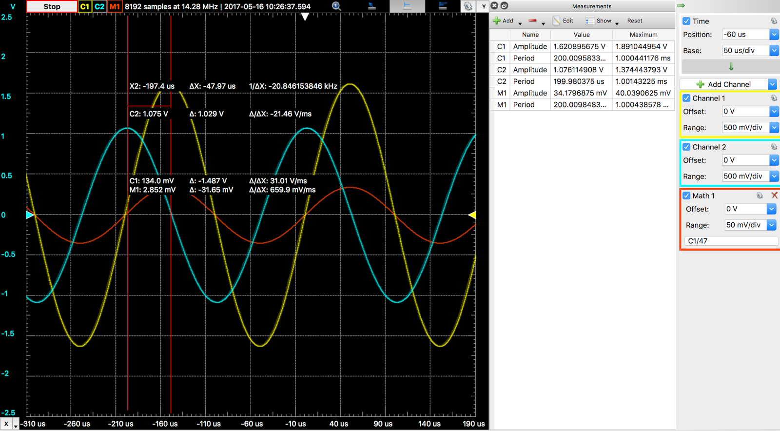
3.  A 47ohm resistor will be connected in series with a a resistor R = 98.8ohms. Then the resistor will be changed to a capacitor C=.092uf with the 47 ohm resistor still connected in series. Finally, the capacitor will changed out to an inductor L = 1mH with the 47 ohm resistor still in series. The oscilloscope measures the voltage across the component mentioned, the current which is mathematically written as Voltage across the 47ohm resistor divided by the resistor value, I=Vr/R. The measurements can be seen below. The voltage input for all experiments are v(t) = 2cosωt. we also acquire our frequency by ω=2πf where f is 1kHz,5KHz and 10KHz

Figure 6. 1KHz with resistor

Figure 7. 5KHz with resistor

Figure 8. 10KHz with resistor

Figure 9. 1KHz with inductor

Figure 10. 5KHz with inductor

Figure 11. 10 KHz with inductor

Figure 12. 1KHz with capacitor

Figure 13. 5KHz with capacitor

Figure 14. 10KHz with capacitor

4. Out theoretical results are compared to experimental results as seen in figure 15.

Figure 15. Theoretical and experimental results

Learning Outcome: 

The lab requires finding the impedance Z of three circuits that contain a resistor Resistance = 46.9士 .05Ω  to another resistor R = 98.8士.05Ω, resistor Resistance = 46.9士 .05Ω, connected to an inductor  L = 1mH, and resistor Resistance = 46.9士 .05Ω, connected to a capacitor C = .092uf士.005. We are told to input a sinusoidal voltage of v(t)= 2cos(ωt) where 2 is the amplitude and ω is the frequency. When calculating the theoretical impedance, we must point out that our given freqencies of 1kHz, 5kHz, and 10kHz must be changed to rad/sec, so the equation ω=2πf will be used. Though, for the experiment, the frequency in hertz is used. Calculations for impedance for each set up can be seen in figure 15, as well as the current in the form of time domain. We are able to compare our theoretical and experimental amplitudes for the current which shows a percent differene of less than 6% for all sets up meantioned above. We can see based on out theoretical calculations that for the resistor connected in series with another resistor that voltage is in phase with current not matter whhat the freqnency. However, for the circuits that are connected with the resistor in series with the inductor or capacitor are different. For the inductor, the voltage leads the current and for the capacitor, the current lead the current. We ere unable to find the phase difference between the current and the voltages. 

Phasors: Passive RL Circuit Response Lab

Objective:
We entered the world of alternating voltage where we have sinusoids to deal with. For instance, if we have a v(t)=Vsinwt, the v is the amplitude (vertical stretch), w is the angular frequency in rad/sec(stretches the wave), and can have a phase shift or vertical shift.  We can also see if we graph two sinusoidal voltages where one has a phase shift, we can see which voltage leads or lags the other. When we deal with sinusoids and adding them, we can use a graphical technique which makes calculations easier. the horizontal axis represent the magnitude of cosine and vertical axis represent the magnitude of the sine. Steinmetz is the father of AC analysis and now sinusoids can be expressed in terms of phasors. Phasors is a complex number that represents the amplitude and phase of a sinusoid. Our complex number can be written or represented in three ways: rectangular form, polar form, and exponential form.

Group Practice:
1. The image below show how to add two sinusoidal voltages by using a a graphical technique. the length is calculated by calculating the magnitude and finding the angle using trigonometry.

Figure 1. Calculating the magnitude and direction of the sinusoidal voltages.

2. The problem below shows two sinusoidal voltages and are told to find the phase between the two voltages. Using the graphical technique, we can see that the phase is 90-50-10 = 30 degrees.

Figure 2. Calculating the phase between two sinusoidal voltages using the graphical technique.

3. We are given a complex number in rectangular form We are told to rewire it in polar form, therefore, we must find the magnitude, as well as the phase angle using inverse tangent.

Figure 3. Rewriting the complex number from rectangular to polar form. 

3. The image below shows polar form complex number in which will be rewritten in rectangular form. Each piece is transformed and then added up. Finally, they will transformed back to polar form and taking the square root. It is easier to to do the square root when in polar form and easier in rectangular form when adding.

Figure 4. The image below shows the order in which we evaluate the complex numbers. 

4. We are given a phasor and must find the sinusoidal representation of the phasors. In order to this, we need to convert the phasor in polar form and then multiply as seen below. Finally, we can convert it to a time domain.

Figure 5. Transforming a phasor into a time domain.

5. We are told to find a current trough a .1H inductor with a sinusoidal voltage. In order to achieve this, we must know the frequency domain for an inductor.  and transforming the equations into polar form. When in polar form, we can find the current by dividing the polar form complex number. It is also easier to have this in polar form since it is easier to divide. Finally, it is then transformed to a time domain.

Figure 6. Finding the current in the form a time domain given a sinusoidal voltage and inductance. 

Phasors: Passive RL Circuit Response Lab Procedures and Results:
1. The lab involves measuring the gain and phase response of an RL circuit comparing them our theoretical values. As seen in figure 8, we calculated our theoretical gain difference and phase difference. We calculated a phase difference of 45 degrees for corner frequency. The gain difference=.015. We also calculated the high frequency gain=.02117 and the low frequency gain=.002117. Most importantly, we calculated the cut of frequency = 47000 rad/sec. Though we must keep in mind that we need to divide by 2π. so the cut of frequency in hertz is, Cut of frequency = 7480 Hz. This value will be used for the lab when entering the sinusoidal voltage of 1 v with the frequencies we are told to use.

Figure 7. The actual circuit with equations of gain and phase difference

Figure 8.  Measurements for cut of frequency.

2. We measure the actual resistance of the resistor R =47.5Ω and the conductor is assumed to be L=.001H since there is not way of measuring it. The actual set can be seen in figure 9 as seen below.

Figure 9. Actual circuit set up 

3. We will now measure the input voltage, current, and voltage across the inductor. From the graph values collected we will calculate the Gain and phase at each frequency. the vales can be measure by looking at figure 10 and 11.

Figure 10. Measuring the gain.

Figure 11. Measuring the phase.

4. The results can be seen below with the help of figure 10 and 11:

GAIN = amplitude of I/amplitude of V, PHASE = ∆T/T * 360

Figure 12. LOW FREQUENCY

Figure 13. HIGH FREQUENCY

5. The results can be seen below for theoretical and experimental values

Figure 14. Experimental and theoretical values

Learning Outcome:

The objective of the lab is to compare our experimental and theoretical results for gain and phase change. Our theoretical results are: cut off frequency, ωc = 47000rad/sec, gain = .02117 at low frequency, gain = .002117 at high frequency, gain = .015 at corner, phase shift = 5.71° at low frequency, phase shift = 84.3° at high frequency, phase shift = 45° at corner frequency. It is important to note when entering the frequency for the input sinusoidal voltage of 1v, we converted the cut off frequency into herts by dividing the value by 2π. So, the frequency in hertz is ωc=7480Hz. The input voltage frequencies were ω=ωc/10=748Hz(LOW), ω=ωc*10=74.8kHz(HIGH), ω=ωc=7480Hz(CORNER). We now compared with our experimental measurements by following figure 10 and 11 where gain = amplitude of voltage out/ amplitude of voltage in. Phase is calculated by the change in period from voltage input and voltage output divided by the period of the voltage input times 360. We acquired a gain of .02157 and phase of 7.326 at low frequency. The percent error for gain was 1.89% and shift was 28.2%. This shows that there is a close comparison between theoretical and experimental with a small difference in error. However, the phase shift was not accurately calculated since it was eyeballed using the picture. Unfortunately, due to time, we were unable to measure the high and corner results. 

Series RLC Circuit Step Response Lab

Objective: 
Today's class meeting reflected the idea of RLC circuit. The first focus was handling second order circuits and finding their initial and final conditions of current and voltage in terms of their derivatives. We understood how to find Vc(0), i(0), dv(0)/dt, di(0)/dt, ic(inf), and vc(inf). When determining the initial conditions we must keep in mind that v and i are defined strictly according to the passive sign convention and that capacitor voltage and inductor current is always continuous. RLC circuits are called second order circuits and when solved found that we can get three types of solutions: if alpha>Wo->overdamped case, if alpha=Wo->critically damped, alpha<Wo->underdamped. For different case, we keep in mind of using different equations.

Group Practice:
1.  The problem below shows how to find the initial and final values, most importantly the derivatives, dv/dt and di/dt.

Figure 1. Finding the initial and final conditions of an RLC circuit.

2. The problem below considers a source free series RLC circuit. By applying KVL we acquire a second order differential equation. We would then let i= Ae^st since the solution will be of an exponential form. By replacing the i and taking the derivative we can see that get a quadratic equation. Solving for s will give us the roots and can compacted by replacing the R/2L=alpha and 1/sqrt(LC)= omega. 

Figure 2. Process of solving a second order differential equation. 

3. The problem below shows how to solve for alpha and omega. We then consider whether it is overdamped, critically damped, or underdamped case.

Figure 3.  Given a circuit, we find alpha and omega and state the response.

4. The problem below shows how to find for the constants A1 and A2 for a parallel circuit.

Figure 4. We found the constants given some initial conditions of voltage.

Series RLC Circuit Step Response Lab and Procedures:
1. As part of the pre lab, we are required to calculate the undamped natural frequency and the neper frequency as seen in figure 6. We see that omega which is the undamped natural frequency is bigger than the neper frequency. This means that the we have an underdamped case.

Figure 5. Schematic for a series RLC Circuit

Figure 6. Finding the case of the circuit. Based on our results. It is underdamped. 

2. We expect the response for this case to be exponentially damped and oscillatory in nature. An example can be seen in figure 7.

Figure 7. Expected measurement response.

3. Before we start making the circuit, we measure our components: Resistor = 1.8 ohms, Inductor = 1mH, and capacitor 92.2 nF. We build a series RLC circuit and input a 2V step input with a low frequency. We also measure the voltage of the capacitor using the oscilloscope. However, we measure our theoretical values for the following: undamped natural frequency, damped natural frequency, damping ratio, rise time, overshoot, and DC gain. The calculations can be seen in figure 8 and the actual set up in figure 9.

Figure 8. Calculations

Figure 9. Actual set up for a series RLC circuit.

4. We measure the voltage across the capacitor and acquired the graph as seen in figure 10. 

Figure 10. the unexpected voltage output for the capacitor.

Series RLC Circuit Step Response Lab and Learning Outcome:
The first step of the experiment is to calculate our undamped natural and neper frequency. However, we first measure our actual components for the series RLC circuit which are , R=1.8ohms, L = 1mH, and C = 92.2nF. We get values of omega= and alpha = using the equations seen in figure 8 above . Based on our results, we noticed that the our alpha is smaller than our omega which means that the solution will be of an underdamped case. We also calculated the following: underdamped natural frequency=omega = 104,144, neper frequency=alpha=900, damping ratio=Z=.00864, and damped natural frequency =omega d = 104,140. The rise time is calculated by looking at the time in which the process first reaches the steady state value. and overshoot is calculated by acquiring the upper amplitude and dividing by the lower amplitude of the underdamped case. From out theoretical value we will compare with our experimental results. However, we did not correctly acquired our expected graph for the voltage as seen in figure 10. As a result, we were unable to compare our theoretical values with our experimental. The next step is to to modify our circuit so that the circuit becomes critically damped. The only way in which this can occur is if the underdamped natural frequency equals the neper frequency. Since we are unable to change natural frequency or DC gain, then the only way is to change the resistance to value where alpha will equal omega.

Inverting Differentiator Lab

Objective:
We covered integrators and differentiator op amps which involve resistors and capacitors In order to create an ideal integrator, we replace the resistor feedback with a capacitor for an inverting amplifier. We can find the current  through nodal analysis at the negative terminal which has a voltage of 0v and can calculate an equation based on the voltage input and output (Vout(t) -V(0) =-1/RC int(Vin(t)dt). To create an differentiator, we can replace the input resistor with a capacitor in an inverting amplifier. the equation calculated is Vout = -RCdvi/dt. Differentiators are unstable and rarely used because of exaggerated noise. We also covered the idea of switching functions and others. In the end, we covered step response of RC and RL circuits.

Group Practice:
1. We are required to find the voltage by using the equation as seen in figure 1. In order to acquire the voltage, we will integrate the current. The voltage graph is then plotted.

Figure 1. Finding the voltage given a current impulse

Inverting Differentiator Lab Procedures and Results:
1. For pre lab, we are required to find an equation of an output voltage as a function of input voltage based on the differentiator op amp. The final equation can be seen in figure 2. We are required to find the frequency needed in the experiment by having the voltage gain Vout/Vin = 1. Therefore, we acquire a frequency of f =2344Hz as long as A = 1, R = 680ohms, and C = 1microfarad.

Figure 2. Calculations for the frequency. 

2. Before, the circuit built, we first measure the actual capacitance of the capacitor and the resistance of the resistor. The resistor has a resistance of R=680 +/-.005 ohms and capacitor of capacitance of C= .945+/-.0005 microfarad. The final build op amp differentiator can be seen in figure 3 & 4. We make sure that we create a voltage sine input with frequencies of 100Hz, 250Hz, 500Hz and measure the voltage output with oscilloscope.

Figure 3. Over all set of op amp differentiator.

Figure 4. Close visual of op amp differentiator.

5. We measured the voltage output when the voltage input with a frequency of 100 Hz was set as seen in figure 5. The voltage output at 250 Hz can be seen in figure 6 and 500 Hz in figure 7.

Figure 5. Voltage output at 100Hz

Figure 6. Voltage output at 250 Hz

Figure 7. Voltage output at 500 Hz

6. We then calculate the theoretical voltage output which can be seen in figure 8 and compare them to our experimental voltage output measurements by looking at the amplitude of the sin wave. We can that they close to each other with percent error less that 3%. We also notice that fussiness throughout the curves.

Figure 8. Comparison of theoretical and experimental voltage outputs for a differentiator op amp. 

Summary of Inverting Differentiator Lab and Learning Outcome:
The lab required us to calculate or find the voltage output as a function of the input voltage in the form of a sinusoid. Since we are dealing with an inverting differentiator, we use the applicable equation derived from earlier in class. We are looking for gain of or Vout/Vin = 1. As a result we can find the frequency in which we can acquire this gain. The frequency we calculated is f = 234 Hz. We also noted that the amplitude of the sinusoidal input will be 1 V and an offset of 0. The measurements of resistor and capacitor are R=680 +/-.005 ohms and C= .945+/-.0005 microfarad. The frequency that we will use to will fall within our frequency of f =234Hz. The frequencies used in the experiment are 100Hz, 250 Hz,  and 500 Hz. From this we noticed that our amplitude increased which means that our voltage output is just proportional to the frequency. We do notice some fussiness in our measurements. Overall when we compared our theoretical and experimental measurements, we see that there is 1.09% error at 100Hz,  2.99% at 250Hz, and 1.69% at 500Hz. The equation for an inverting differentiator hold true since the percent error is relatively low.

Passive RC/RL Natural Response Lab

Objective:
We covered the idea that the equivalent inductance of inductors connected in series or parallel is similar to the idea of resistors in which they add in series and are inversely added when they are in parallel. The goal is to understand what is happening in RC and RL circuit and Passive RC/RL Natural Response Lab will help us do that. For RC circuit, the capacitor initially acts like a wire but after a long time, it acts like an open switch. We will use the equations i(t) = Io*e(-t/RC) or v(t)=Vo*e(-t/RC). For an RL circuit, initially, the inductor opposes rapid change so it acts like an open switch but after a long time, its acts like an ordinary wire. The equations that we will use are i(t)=Io*e(-tR/L).

Group Practice:
1. We are given a first order differential equation in which we must solve the Voltage of the capacitor in terms of time. We see that tau is the resistance times the capacitance so it can be replaced by tao in equation as seen below in Figure 1. We show that the voltage of the capacitor is 1% of the initial voltage in order to see that the voltage of the capacitor drops close to 0. We will use the idea that
t =5*RC which is the time that the capacitor discharges and we use it as an approximation of time discharge.

Figure 1. Using 1st order linear differentiation to solve for voltage across a capacitor

2. Figure 2 tells us to find the max switch frequency and we can find this by finding the time in which the capacitor discharges which is t=5*RC = .005sec. the Frequency= 1/t = 200Hz which is a low pass filter.

Figure 2. Find the max switch frequency of an RC circuit.

Passive RC Natural Response Lab Procedures and Results:

1. The pre lab requires us to calculate the initial voltage of the capacitor and we do this by showing that Vc = Vo(R2/R1+R2) = 3.438V assuming that capacitor acts as open circuit when the capacitor is fully charged. The voltage across the R2 is the voltage of the capacitor since they are parallel to each other.

Figure 3. Initial voltage for the capacitor calculations.

2. We then find the time constant where tau= RC = .0484sec for circuit a as seen in figure 4. The time it takes to discharge is t = 5*.0484 = .242sec  based on figure 4 circuit a. We find the time constant were tau = C*(R1*R2/R1+R2) = .01513sec for circuit b in figure 4. We find the time when discharging from figure 4b by multiplying by 5 since we assume the time of discharging is t = 5*tau = .0756sec.

Figure 4. Schematics for circuits that will be used in the lab. 

3. We construct the circuit as seen in figure 5 and measure the actual resistance of the resistors which are R1= .95K+/-.05 and R2= 2.13+/-.05. The analog discovery will measure the voltage across the capacitor when quickly disconnecting the power supply from the circuit, thus following the procedure from figure 4 a.

Figure 5. Actual circuit set up

Figure 6. The visual discharge of a capacitor when the circuit is suddenly disconnected from the voltage source.

4. The next step is to turn off the voltage source which will act as a wire. The procedure schematic can be seen in figure 4 b. The visual result can be seen below.

Figure 7. The visual discharge of the capacitor when the circuit is turned off instead of suddenly being disconnected.

5. We also measured the time of the voltage charge of the capacitor which can be seen in figure 7.

Figure 8. The visual charge of the capacitor. 

6. When suddenly disconnecting the voltage source, we measured a time of discharge t =.270 sec. When the voltage source was turned off, we acquired a time discharge of t = .07sec. There is a percent error of %error=(.270-.242)/.242 *100 = 11.5 % when suddenly disconnecting the voltage source. There is a percent error of %error = (.07-.0756)/.0756 *100 = 7.41%

7. The next step is to use a square wave with an amplitude of 2.5V and an offset of 2.5V that oscillates between 0V and 5V and a frequency of 1Hz. 

Passive RL Natural Response Lab Procedures and Results:
1. We are given an inductor and we must calculate the value of the inductor L. In order to calculate the the value of the inductor, we must use the equations i(t) = Io*e(-tR/L). The first step is to use the same setup as the passive RC Natural Response Lab and calculate the voltages across R1 and R2. With these measurements we can find the current that flow in R1. We can then use the equation Vr= Io*R*e(-tR/L) and manipulate it so that we can solve for L

Summary of Passive RC/RL Natural Response Lab and Learning Outcome:
The main focus of the Passive RC Natural Response Lab is to calculate and compare the time it takes to discharge a capacitor when the circuit is suddenly disconnected and turned off. We can assume that when the circuit is suddenly disconnected, the resistor which is connected to the voltage source is neglected since there is no current flowing through the wire. Therefore, we can assume that the time it takes to discharge the capacitor will be higher than when the voltage source is simply turned off. Based on our theoretical calculations, we acquire a time of discharge of t = 5*.0484 = .242sec when the voltage source is suddenly turned off. We acquire a time of discharge of t = 5*tau = .0756sec when the voltage source is simply turned off. We approximated the experimental time as seen in figure 5 and 6. The time of discharge when voltage source is suddenly tuned off is t = .270sec and when voltage source is turned off, t = .07sec. We calculated the percent error when disconnecting the voltage source of 11.5% error and when the voltage was simply turned off 7.41% error. Our theoretical time falls within our experimental results since the percent error is low. We were unable to to calculate the experimental time constant since we did not measure the capacitance of the capacitor. However, out theoretical time constant is Tau = .0484 sec for sudden disconnection and Tau = .01513sec for turned off power source. We were unable to finish the RL natural response Lab but have a sense on how to do it. The idea was to measure the voltage across the both the resistors and use those voltages to acquire the current and finally use the equationVr= Io*R*e(-tR/L).